Image Classification with TensorFlow

1 Introduction
This article discusses the task of multi-class image classification using TensorFlow. The main topics covered include loading image data, data augmentation, model training, transfer learning, and the use of TensorBoard. All the code examples are based on TensorFlow v2.8.0. The code can be run on Google Colab, which provides free GPU acceleration to speed up the training process.
2 Image Processing
Loading the original image data containing 10 classes of objects:
import zipfile
import os
import matplotlib.pyplot as plt
import datetime

import tensorflow as tf
from tensorflow.keras.preprocessing.image import ImageDataGenerator
from tensorflow.python.ops.gen_array_ops import shape
from tensorflow.keras import layers

!wget https://storage.googleapis.com/ztm_tf_course/food_vision/10_food_classes_all_data.zip

# Unzip the downloaded file
zip_ref = zipfile.ZipFile("10_food_classes_all_data.zip", "r")
zip_ref.extractall()
zip_ref.close()

# Function for processing images
def load_and_process_image(file_name, img_shape=224):
  """
  Read an image and process it, reshape it to (img_shape, img_shape, color_channels)
  """
  # Read the image
  img = tf.io.read_file(file_name)

  # Decode the read file into a tensor
  img = tf.image.decode_image(img)

  # Resize the image
  img = tf.image.resize(img, size=[img_shape, img_shape])

  # Scale the image
  img = img/255.

  return img

# Function to display files
def list_files(startpath):
    for root, dirs, files in os.walk(startpath):
        level = root.replace(startpath, '').count(os.sep)
        indent = ' ' * 4 * (level)
        print('{}{}/'.format(indent, os.path.basename(root)))
        subindent = ' ' * 4 * (level + 1)
        for f in files:
            print('{}{}'.format(subindent, f))

# Walk through the 10_food_classes directory and list the number of files
for dirpath, dirnames, filenames in os.walk("10_food_classes_all_data"):
  print(f"There are {len(dirnames)} directories and {len(filenames)} images in '{dirpath}'.")
From the output, we can see that the data contains images of various food items such as ice cream, steak, pizza, etc.
There are 2 directories and 0 images in '10_food_classes_all_data'.
There are 10 directories and 0 images in '10_food_classes_all_data/test'.
There are 0 directories and 250 images in '10_food_classes_all_data/test/chicken_wings'.
There are 0 directories and 250 images in '10_food_classes_all_data/test/pizza'.
There are 0 directories and 250 images in '10_food_classes_all_data/test/grilled_salmon'.
There are 0 directories and 250 images in '10_food_classes_all_data/test/sushi'.
There are 0 directories and 250 images in '10_food_classes_all_data/test/fried_rice'.
There are 0 directories and 250 images in '10_food_classes_all_data/test/ice_cream'.
There are 0 directories and 250 images in '10_food_classes_all_data/test/chicken_curry'.
There are 0 directories and 250 images in '10_food_classes_all_data/test/hamburger'.
There are 0 directories and 250 images in '10_food_classes_all_data/test/ramen'.
There are 0 directories and 250 images in '10_food_classes_all_data/test/steak'.
There are 10 directories and 0 images in '10_food_classes_all_data/train'.
There are 0 directories and 750 images in '10_food_classes_all_data/train/chicken_wings'.
There are 0 directories and 750 images in '10_food_classes_all_data/train/pizza'.
There are 0 directories and 750 images in '10_food_classes_all_data/train/grilled_salmon'.
There are 0 directories and 750 images in '10_food_classes_all_data/train/sushi'.
There are 0 directories and 750 images in '10_food_classes_all_data/train/fried_rice'.
There are 0 directories and 750 images in '10_food_classes_all_data/train/ice_cream'.
There are 0 directories and 750 images in '10_food_classes_all_data/train/chicken_curry'.
There are 0 directories and 750 images in '10_food_classes_all_data/train/hamburger'.
There are 0 directories and 750 images in '10_food_classes_all_data/train/ramen'.
There are 0 directories and 750 images in '10_food_classes_all_data/train/steak'.
Extract all the labels:
class_names = os.listdir("10_food_classes_all_data/train/")
train_dir = "10_food_classes_all_data/train/"
test_dir = "10_food_classes_all_data/test/"
In addition, use the TensorFlow's tensorflow.keras.preprocessing.image.ImageDataGenerator API to process and enhance the images. In short, this API can automatically generate labels for images based on the file directory and enhance the images according to the specified operations. Note that "data augmentation can only be used on the training set."
train_datagen_augmented = ImageDataGenerator(rescale=1/255.,
                                             rotation_range=20, # Rotate images
                                             shear_range=0.2, # Shear images
                                             zoom_range=0.2, # Zoom images
                                             width_shift_range=0.2, # Shift images horizontally
                                             height_shift_range=0.2, # Shift images vertically
                                             horizontal_flip=True) # Flip images horizontally

train_datagen = ImageDataGenerator(rescale=1/255.)

test_datagen = ImageDataGenerator(rescale=1/255.)

# Generate the datasets
train_data = train_datagen_augmented.flow_from_directory(train_dir,
                                                        target_size=(224,224),
                                                        batch_size=32,
                                                        shuffle=True)

test_data = test_datagen.flow_from_directory(test_dir,
                                              target_size=(224,224),
                                              batch_size=32)
3 Modeling
3.1 Baseline Model
First, create a convolutional neural network as the baseline model:
# Plot the training curves
def plot_loss_curves(history):
  """
  Returns separate loss curves for training and validation metrics.
  """
  loss = history.history['loss']
  val_loss = history.history['val_loss']

  accuracy = history.history['accuracy']
  val_accuracy = history.history['val_accuracy']

  epochs = range(len(history.history['loss']))

  # Plot loss
  plt.plot(epochs, loss, label='training_loss')
  plt.plot(epochs, val_loss, label='val_loss')
  plt.title('Loss')
  plt.xlabel('Epochs')
  plt.legend()

  # Plot accuracy
  plt.figure()
  plt.plot(epochs, accuracy, label='training_accuracy')
  plt.plot(epochs, val_accuracy, label='val_accuracy')
  plt.title('Accuracy')
  plt.xlabel('Epochs')
  plt.legend()


# Build the model
tf.random.set_seed(42)
tf.keras.backend.clear_session()

cnn_model = tf.keras.models.Sequential([
    layers.Conv2D(filters=10, kernel_size=(3,3), activation="relu",
                  input_shape=(224, 224, 3)),
    layers.MaxPooling2D(pool_size=2),

    layers.Conv2D(filters=10, kernel_size=(3,3), activation="relu"),
    layers.MaxPooling2D(pool_size=2),

    layers.Flatten(),
    layers.Dropout(0.5),
    layers.Dense(10, activation="softmax")
])

cnn_model.compile(loss=tf.keras.losses.CategoricalCrossentropy(),
                optimizer=tf.keras.optimizers.Adam(),
                steps_per_execution=50,
                metrics="accuracy")


def create_tensorboard_callback(dir_name, experiment_name):
  log_dir = dir_name + "/" + experiment_name + "/" + datetime.datetime.now().strftime("%Y%m%d-%H%M%S")
  tensorboard_callback = tf.keras.callbacks.TensorBoard(log_dir=log_dir)
  print(f"Saving tensorboard callback log file to {log_dir}")
  return tensorboard_callback


tf_board_callback =  create_tensorboard_callback

(dir_name="vision_model",
                                                 experiment_name="VGG_base")

history_cnn = cnn_model.fit(train_data,
                            steps_per_epoch=len(train_data),
                            epochs=5,
                            validation_data=test_data,
                            validation_steps=len(test_data),
                            callbacks=[tf_board_callback])

cnn_model.evaluate(test_data)
The output shows the accuracy of the model:
79/79 [==============================] - 12s 148ms/step - loss: 1.8068 - accuracy: 0.3852
[1.8068159818649292, 0.38519999384880066]
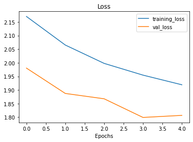
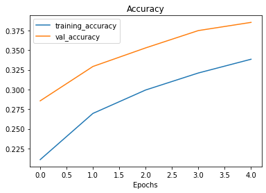
The training curves indicate the trends of the loss and accuracy. If the model is deepened or trained for a longer time, better accuracy can be achieved.
plot_loss_curves(history_cnn)
3.2 Transfer Learning
Another approach to improve model performance is to use transfer learning. Transfer learning involves using a model that has performed very well on other tasks and applying it to your own task. Generally, transfer learning performs better than building a model from scratch because the model architecture and training process have been highly optimized. In this case, we will use the Xception model, which is a highly complex and high-performance model.
# Load the pre-trained Xception model
base_model = tf.keras.applications.xception.Xception(weights='imagenet', include_top=False)
avg = tf.keras.layers.GlobalAveragePooling2D()(base_model.output)
output = tf.keras.layers.Dense(len(class_names), activation='softmax')(avg)
model = tf.keras.Model(inputs=base_model.input, outputs=output)

# Usually, the weights of the pre-trained model are frozen since they have been well-trained and optimized
for layer in base_model.layers:
    layer.trainable = False

optimizer = tf.keras.optimizers.SGD(lr=0.2, momentum=0.9, decay=0.01)
model.compile(loss='categorical_crossentropy', optimizer=optimizer, metrics=['accuracy'])

epochs = 5
tf_board_callback_2 =  create_tensorboard_callback(dir_name="vision_model",
                                                   experiment_name="Xception")

history = model.fit(train_data, epochs=epochs, validation_data=test_data,
                    callbacks=[tf_board_callback_2])

model.evaluate(test_data)
The output shows the improved performance compared to the baseline:
79/79 [==============================] - 31s 390ms/step - loss: 0.5771 - accuracy: 0.8388
[0.5770677924156189, 0.8388000130653381]
You can view the training process in TensorBoard:
# The following commands are for Google Colab only
%load_ext tensorboard
%tensorboard --logdir="vision_model/Xception/20220522-120512/"
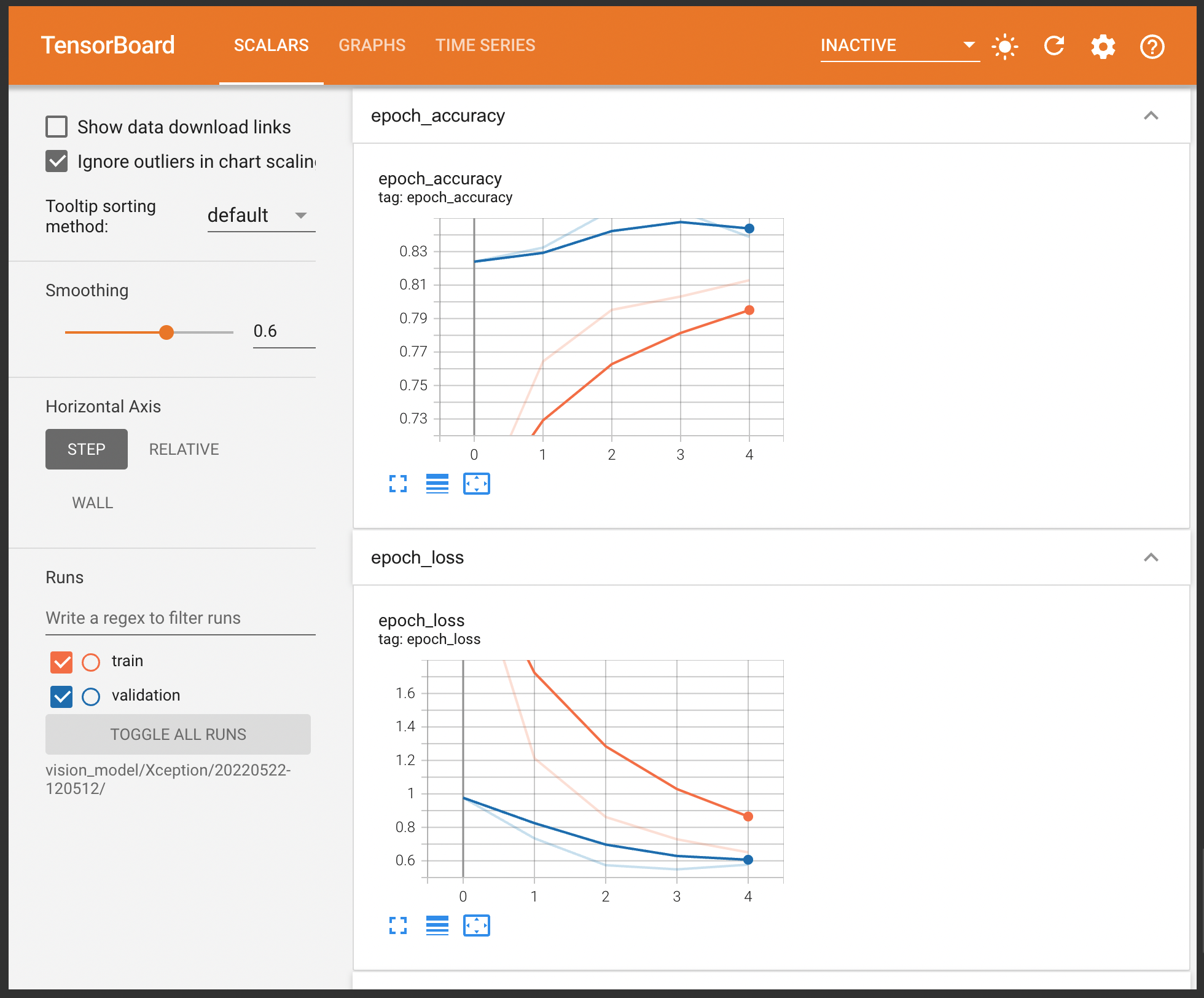
You can also download the computational graph of the model in TensorBoard. The complexity of Xception is significantly higher than the baseline model, explaining its superior performance.

4 Conclusion
This article covers important concepts in image classification tasks using neural networks and important TensorFlow APIs, such as tensorflow.keras.preprocessing.image.ImageDataGenerator, TensorBoard Callback, and how to load pre-trained models. I hope this sharing has been helpful to you. Feel free to leave comments for further discussion!