Univariate Time Series Prediction with TensorFlow

1 Introduction
This article will use TensorFlow to solve time series prediction problems. There is a very detailed but lengthy tutorial on the TensorFlow official website, so this article will focus on the core content of univariate time series prediction in an easy-to-understand way.
2 Bitcoin Price Dataset
2.1 Get Data
This article uses Bitcoin historical price data (from October 2013 to May 2021) for prediction. Please note that this article does not constitute investment advice!
!wget https://raw.githubusercontent.com/mrdbourke/tensorflow-deep-learning/main/extras/BTC_USD_2013-10-01_2021-05-18-CoinDesk.csv

import pandas as pd
import matplotlib.pyplot as plt
import os
import tensorflow as tf
from tensorflow.keras as layers

df = pd.read_csv("/content/BTC_USD_2013-10-01_2021-05-18-CoinDesk.csv",
                 parse_dates=["Date"],
                 index_col=["Date"]) # Parse the date column

df.tail()
Returns:
| Date | Currency | Closing Price (USD) | 24h Open (USD) | 24h High (USD) | 24h Low (USD) |
|---|---|---|---|---|---|
| 2021-05-14 | BTC | 49764.132082 | 49596.778891 | 51448.798576 | 46294.720180 |
| 2021-05-15 | BTC | 50032.693137 | 49717.354353 | 51578.312545 | 48944.346536 |
| 2021-05-16 | BTC | 47885.625255 | 49926.035067 | 50690.802950 | 47005.102292 |
| 2021-05-17 | BTC | 45604.615754 | 46805.537852 | 49670.414174 | 43868.638969 |
| 2021-05-18 | BTC | 43144.471291 | 46439.336570 | 46622.853437 | 42102.346430 |
Take the closing price for prediction:
bitcoin_prices = pd.DataFrame(df["Closing Price (USD)"]).rename({"Closing Price (USD)":"Price"},axis=1)
bitcoin_prices.head()
| Date | Price |
|---|---|
| 2013-10-01 | 123.65499 |
| 2013-10-02 | 125.45500 |
| 2013-10-03 | 108.58483 |
| 2013-10-04 | 118.67466 |
| 2013-10-05 | 121.33866 |
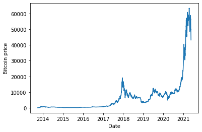
View the bitcoin price trend with a chart:
plt.plot(bitcoin_prices["Price"])
plt.ylabel("Bitcoin price")
plt.xlabel("Date")
2.2 Create Time Windows
The expected data format is [0,1,2,3,4,5,6] -> [7], that is, use the prices from the past seven days to predict the price for the next day. Here, use the window division provided by TensorFlow, timeseries_dataset_from_array.
timesteps = bitcoin_prices.index.to_numpy()
prices = bitcoin_prices["Price"].to_numpy()

HORIZON  = 1 # Predict the price for the next day
WINDOW_SIZE = 7 # Use prices from the previous 7 days

input_data = prices[:-HORIZON]
targets = prices[WINDOW_SIZE:]
dataset = tf.keras.preprocessing.timeseries_dataset_from_array(
    input_data, targets, sequence_length=WINDOW_SIZE)
for batch in dataset:
  inputs, targets = batch
  assert np.array_equal(inputs[0], prices[:WINDOW_SIZE])
  assert np.array_equal(targets[0], prices[WINDOW_SIZE])

  print(f"First Input:{inputs[0]}, Target:{targets[0]}")
  print(f"Second Input:{inputs[1]}, Target:{targets[1]}")

  break
Returns as follows, the data has been correctly transformed as expected.
First Input:[123.65499 125.455   108.58483 118.67466 121.33866 120.65533 121.795  ], Target:123.033
Second Input:[125.455   108.58483 118.67466 121.33866 120.65533 121.795   123.033  ], Target:124.049
2.3 Split Data
Use time to split the training set and validation set. No test set is included as examples only. In actual use, one can operate according to needs.
# Because tf.keras.preprocessing.timeseries_dataset_from_array returns a batched dataset, unbatch first for easy data splitting
dataset = dataset.unbatch()

test_split = 0.2
split_index = int(len(list(dataset)) * (1-test_split))

# After splitting, split the batch again, add one dimension, otherwise it does not meet the data dimension requirements of the model
train_dataset = dataset.take(split_index).batch(batch_size=32)
test_dataset = dataset.skip(split_index).batch(batch_size=32)
3 Modeling
Since this article does not pursue the ultimate prediction accuracy, only a fully connected layer is used to build the model, the code is as follows:
tf.random.set_seed(42)
tf.keras.backend.clear_session()

# 1. Build the model
model = tf.keras.models.Sequential(
[
 layers.Input(WINDOW_SIZE),
 layers.Dense(128, activation="relu"),
 layers.Dense(HORIZON, activation="linear")
]
, name="model_dense_base")

# 2. Compile the model
model.compile(loss='mae',
                optimizer=tf.keras.optimizers.Adam(),
                metrics=['mae'])


# Create callback to save the best performing model checkpoint
def create_model_checkpoint(model_name, save_path="model_checkpoint"):
  return tf.keras.callbacks.ModelCheckpoint(filepath=os.path.join(save_path, model_name),
                                            verbose=0,
                                            save_best_only=True)

# 3. Train the model
model.fit( train_dataset,
            epochs=100,
            verbose=0,
            validation_data=test_dataset,
            callbacks=[create_model_checkpoint(model_name=model.name)]
            )
Load the best performing model back for evaluation:
model = tf.keras.models.load_model("model_checkpoint/model_dense_base")
model.evaluate(test_dataset)
The result shows the average absolute error (MAE), indicating that the predicted price is more than 700 US dollars different from the real price on average.
18/18 [==============================] - 1s 6ms/step - loss: 759.4327 - mae: 759.4327
[759.4326782226562, 759.4326782226562]
Considering that the model structure is very simple, there is room for improvement in the results, and it can be predicted more accurately by optimizing according to this process.
4 Summary
This article did a benchmark for univariate time series prediction tasks, in which the TensorFlow tf.keras.preprocessing.timeseries_dataset_from_array API simplified a lot of work on processing time windows. In the future, we will continue to discuss TensorFlow's prediction of time series tasks.