Decision Tree Overview

1 Introduction

Decision tree is very classical machine learning model that can be used to solve many classification and regression problems in daily work. Many more advanced machine learning models are also built based on decision trees. Today, let's review some of the most important technical details in decision trees to solidify the foundation and correctly apply decision trees.

2 Important Algorithm Details

2.1 Making Predictions

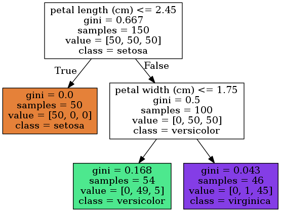
The example displays a decision tree with a depth of 2, showing the process and conclusions of decision-making. For 150 sample points, at the root node, the decision tree divides the data into two parts based on whether the petal length is less than 2.45 cm. The samples with a petal length less than 2.45 cm are classified as setosa, and the ones with a petal length greater than 2.45 cm are further classified based on whether the petal width is less than 1.75 cm. The ones that are less than 1.75 cm are considered versicolor, and the ones that are greater than 1.75 cm are considered virginica.

The "samples" in the graph represent the number of samples in each category. For example, in the left leaf node at depth 1, "samples=50" means that there are 50 samples with a petal length less than 2.45 cm. The "value" represents the distribution of training data in the current node. For example, in the green left node at depth 2, "[0, 49, 5]" represents that there are 0 setosa, 49 versicolor, and 5 virginica in this node, totaling 54 samples.

2.2 Basis for Predictions

In the decision tree example, there is another important indicator called "Gini impurity," which measures the impurity of the current node. Intuitively, when all the samples in a node belong to the same class, the purity of the node is the highest, and the Gini impurity is 0. The definition of "Gini" is as follows:

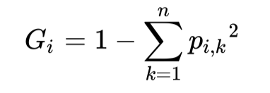
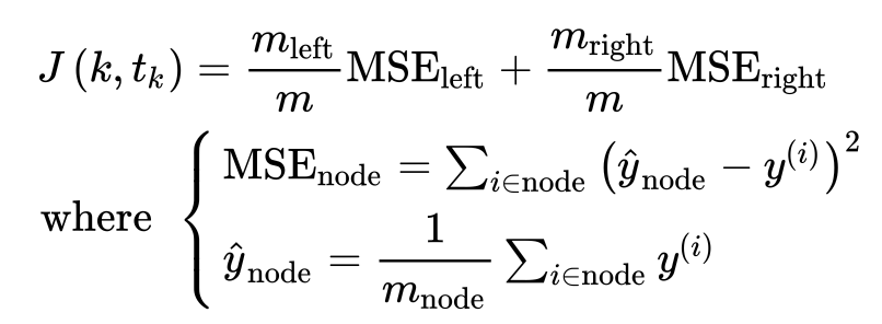
where Pi,k is the proportion of samples in class k in node i. In the commonly used Python machine learning library Scikit-Learn (v0.24.2), when implementing the classification and regression tree (Classification and Regression Tree, CART), in the process of selecting split nodes, the basis for the decision tree to select split nodes and thresholds is related to . Its optimization objective (loss function) is as follows:

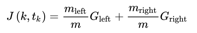
Gini in The CART algorithm will do a greedy search (Greedy Search), start splitting from the root node, and search for features and thresholds that can be effectively reduced in the layer-by-layer child nodes , until the number of split layers reaches the maximum depth (defined by the max_depth parameter) or has been found Less than Ginithe node that can be reduced. Intuitively, finding the best tree is an NP-complete problem, so the algorithm will only find a relatively good solution in the end, not the best solution.

In addition to "Gini," entropy can also be used to measure the effectiveness of splitting nodes and to quantify the degree of disorder. In a decision tree, when all samples in a node belong to the same class, the entropy value is 0. The definition of entropy is as follows:

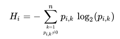
where Pi,k is the proportion of samples in class k in node i. In Scikit-Learn (v0.24.2), when using the DecisionTreeClassifier class, you can set the criterion parameter to entropy to use entropy as the measure. However, the difference between using Gini and entropy is usually not significant. The main difference is that the Gini calculation is faster, and using Gini will make the tree concentrate the samples more in the nodes, while using entropy will make the distribution of samples in the tree more balanced.

2.3 Preventing Overfitting

Decision trees themselves have almost no assumptions and do not rely on feature scaling, but the model itself needs constraints to prevent overfitting. Regularization can be achieved by controlling the model parameters. Taking the DecisionTreeClassifier class in Scikit-Learn (v0.24.2) as an example, the following parameters are commonly used for regularization to prevent overfitting:

• max_depth: The maximum depth of the tree. The default value is None, which means there is no maximum depth limit for the tree.
• min_samples_split: The minimum number of samples required to split an internal node. The default value is 2.
• min_samples_leaf: The minimum number of samples required to be at a leaf node. The default value is 1.
• min_weight_fraction_leaf: The minimum weighted fraction of the total number of samples required to be at a leaf node. The default value is 0. When class_weight is set and the sample weights are different, this parameter constrains the weighted proportion of samples in the leaf nodes, similar to min_samples_leaf, but expressed as a proportion.
• max_features: The number of features to consider when looking for the best split. The default is to consider all features. Note that the decision tree will not stop searching for a valid split until it has searched the number of features specified by max_features, even if it exceeds that value.
• max_leaf_nodes: The maximum number of leaf nodes. The default value is None.
• min_impurity_decrease: The minimum impurity decrease required to split a node. The default value is 0.

Usually, increasing the min_ parameters or decreasing the max_ parameters helps with regularization of the decision tree.

2.4 Regression Task

In Scikit-Learn (v0.24.2), you can use the DecisionTreeRegressor class to perform regression tasks.

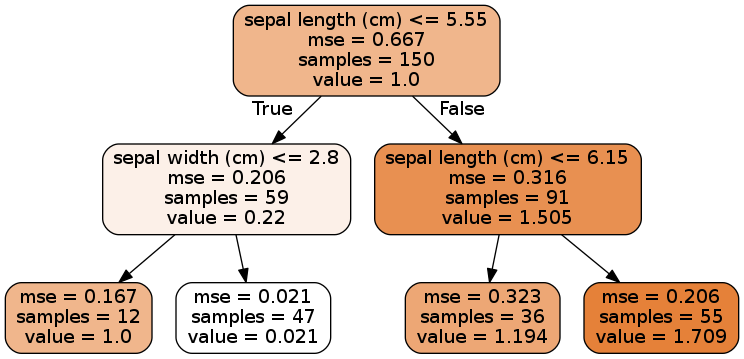
In regression tasks, the predicted value at a leaf node is the mean of the target values of the samples in that leaf node. The implementation of the CART algorithm for regression is similar to classification, but the optimization objective is to minimize the mean squared error (MSE) between the predicted values and the target values.

The model parameters for regression trees are similar to those for classification trees, and you can use similar techniques to prevent overfitting.

2.5 Other Important Attributes

In the Scikit-Learn implementation, the feature_importances_ attribute of a decision tree can show the importance of features. It is based on the reduction in the criterion measure for each feature and returns normalized values. If you have features with a high number of different values (high cardinality features), it is recommended to use sklearn.inspection.permutation_importance.

If you want to manually adjust the tree, such as changing the splitting threshold, you can use sklearn.tree._tree.Tree.

3 Summary

Decision trees perform well for both classification and regression tasks. However, they have limitations and weaknesses. For example, they are sensitive to the direction and volatility of the data. These issues cannot be perfectly addressed by a single tree. So, is there a better approach by using multiple trees? In the next discussion, we will talk about random forests!

Here is an example code:

# Dependencies
from sklearn.datasets import load_iris
from sklearn.tree import DecisionTreeClassifier
from sklearn.tree import DecisionTreeRegressor
from sklearn.tree import export_graphviz

import matplotlib.pylab as plt
import numpy as np


# Load sample data
iris = load_iris()
X = iris.data[:, :2]  # Select petal length and petal width as features
y = iris.target

# View data distribution
plt.scatter(X[y == 0, 0], X[y == 0, 1])
plt.scatter(X[y == 1, 0], X[y == 1, 1])
plt.scatter(X[y == 2, 0], X[y == 2, 1])
plt.show()

# Build a decision tree
tree_clf = DecisionTreeClassifier(criterion='entropy', max_depth=2)
tree_clf.fit(X, y)

# Export decision tree graph
export_graphviz(
    tree_clf,
    out_file="iris_tree.dot",
    feature_names=iris.feature_names[:2],
    class_names=iris.target_names,
    rounded=True,
    filled=True
)

# Decision boundary plotting function
def plot_decision_boundary(model, x):
    # Generate coordinate matrices for the

 grid points, resulting in two matrices
    M, N = 500, 500
    x0, x1 = np.meshgrid(np.linspace(x[:, 0].min(), x[:, 0].max(), M), np.linspace(x[:, 1].min(), x[:, 1].max(), N))
    X_new = np.c_[x0.ravel(), x1.ravel()]
    y_predict = model.predict(X_new)
    z = y_predict.reshape(x0.shape)
    from matplotlib.colors import ListedColormap
    custom_cmap = ListedColormap(['#EF9A9A', '#FFF59D', '#90CAF9'])
    plt.pcolormesh(x0, x1, z, cmap=custom_cmap)

# Plot decision boundary
plot_decision_boundary(tree_clf, X)
plt.scatter(X[y == 0, 0], X[y == 0, 1])
plt.scatter(X[y == 1, 0], X[y == 1, 1])
plt.scatter(X[y == 2, 0], X[y == 2, 1])
plt.show()

# View feature importance
print(tree_clf.feature_importances_)